I originally wrote this for a tutorial on learnxinyminutes.com, which attempts to teach you the basics of a new programming language. I use M daily at work, and it gets a lot of unfair criticism in tech journalism for its age and its terseness. I liken M to Python in its usefulness for procedural scripting. It’s also got a very nice debugging tool that lets you pause code mid-execution and inspect the variables as you’re running it. Finally, the database is built right into the language. While I think that setting up a new M environment can be tedious and require a lot of Unix knowledge compared to other programming environments, database replication is very simple compared to some other databases.
Without further ado, here’s an introduction to M:
M, or MUMPS (Massachusetts General Hospital Utility Multi-Programming System) is
a procedural language with a built-in NoSQL database. Or, it’s a database with
an integrated language optimized for accessing and manipulating that database.
A key feature of M is that accessing local variables in memory and persistent
storage use the same basic syntax, so there’s no separate query
language to remember. This makes it fast to program with, especially for
beginners. M’s syntax was designed to be concise in an era where
computer memory was expensive and limited. This concise style means that a lot
more fits on one screen without scrolling.
The M database is a hierarchical key-value store designed for high-throughput
transaction processing. The database is organized into tree structures called
“globals”, which are sparse data structures with parallels to modern formats
like JSON.
Originally designed in 1966 for the healthcare applications, M continues to be
used widely by healthcare systems and financial institutions for high-throughput
real-time applications.
Example
Here’s an example M program to calculate the Fibonacci series:
fib ; compute the first few Fibonacci terms
    new i,a,b,sum
    set (a,b)=1 ; Initial conditions
    for i=1:1 do  quit:sum>1000
    . set sum=a+b
    . write !,sum
    . set a=b,b=sum
Comments
; Comments start with a semicolon (;)
Data Types
M has two data types:
;   Numbers - no commas, leading and trailing 0 removed.
;       Scientific notation with 'E'.
;       Floats with IEEE 754 double-precision values (15 digits of precision)
;       Examples: 20, 1e3 (stored as 1000), 0500.20 (stored as 500.2)
;   Strings - Characters enclosed in double quotes.
;       "" is the null string. Use "" within a string for "
;       Examples: "hello", "Scrooge said, ""Bah, Humbug!"""
Commands
Commands are case insensitive, and have a shortened abbreviation, often the first letter. Commands have zero or more arguments,depending on the command. M is whitespace-aware. Spaces are treated as a delimiter between commands and arguments. Each command is separated from its arguments by 1 space. Commands with zero arguments are followed by 2 spaces.
W(rite)
Print data to the current device.
WRITE !,"hello world"
! is syntax for a new line. Multiple statements can be provided as additional arguments:
w !,"foo bar"," ","baz"
R(ead)
Retrieve input from the user
READ var
r !,"Wherefore art thou Romeo? ",why
Multiple arguments can be passed to a read command. Constants are outputted. Variables are retrieved from the user. The terminal waits for the user to enter the first variable before displaying the second prompt.
r !,"Better one, or two? ",lorem," Better two, or three? ",ipsum
S(et)
Assign a value to a variable
SET name="Benjamin Franklin"
s centi=0.01,micro=10E-6
w !,centi,!,micro

;.01
;.00001
K(ill)
Remove a variable from memory or remove a database entry from disk.
KILL centi
k micro
Globals and Arrays
In addition to local variables, M has persistent variables stored to disk called globals. Global names must start with a caret (^). Globals are the built-in database of M.
Any variable can be an array with the assignment of a subscript. Arrays are sparse and do not have a predefined size. Arrays should be visualized like trees, where subscripts are branches and assigned values are leaves. Not all nodes in an array need to have a value.
s ^cars=20
s ^cars("Tesla",1,"Name")="Model 3"
s ^cars("Tesla",2,"Name")="Model X"
s ^cars("Tesla",2,"Doors")=5

w !,^cars
; 20
w !,^cars("Tesla")
; null value - there's no value assigned to this node but it has children
w !,^cars("Tesla",1,"Name")
; Model X
Arrays are automatically sorted in order. Take advantage of the built-in sorting by setting your value of interest as the last child subscript of an array rather than its value.
; A log of temperatures by date and time
s ^TEMPS("11/12","0600",32)=""
s ^TEMPS("11/12","1030",48)=""
s ^TEMPS("11/12","1400",49)=""
s ^TEMPS("11/12","1700",43)=""
Operators
; Assignment: =
; Unary: + Convert a string value into a numeric value.
; Arthmetic:
; + addition
; - subtraction
; * multiplication
; / floating-point division
; \ integer division
; # modulo
; ** exponentiation
; Logical:
; & and
; ! or
; ' not
; Comparison:
; = equal
; '= not equal
; > greater than
; < less than
; '> not greater / less than or equal to
; '< not less / greater than or equal to
; String operators:
; _ concatenate
; [ contains a contains b
; ]] sorts after a comes after b
; '[ does not contain
; ']] does not sort after
Order of operations
Operations in M are strictly evaluated left to right. No operator has precedence over any other.
You should use parentheses to group expressions.
w 5+3*20
;160
;You probably wanted 65
w 5+(3*20)
Flow Control, Blocks, & Code Structure
A single M file is called a routine. Within a given routine, you can break your code up into smaller chunks with tags. The tag starts in column 1 and the commands pertaining to that tag are indented.
A tag can accept parameters and return a value, this is a function. A function is called with ‘$$’:
; Execute the 'tag' function, which has two parameters, and write the result.
w !,$$tag^routine(a,b)
M has an execution stack. When all levels of the stack have returned, the program ends. Levels are added to the stack with do commands and removed with quit commands.
D(o)
With an argument: execute a block of code & add a level to the stack.
d ^routine    ;run a routine from the begining.
;             ;routines are identified by a caret.
d tag         ;run a tag in the current routine
d tag^routine ;run a tag in different routine
Argumentless do: used to create blocks of code. The block is indented with a period for each level of the block:
set a=1
if a=1 do
. write !,a
. read b
. if b > 10 d
. . w !, b
w "hello"
Q(uit)
Stop executing this block and return to the previous stack level.
Quit can return a value.
N(ew)
Clear a given variable’s value for just this stack level. Useful for preventing side effects.
Putting all this together, we can create a full example of an M routine:
; RECTANGLE - a routine to deal with rectangle math
    q ; quit if a specific tag is not called

main
    n length,width ; New length and width so any previous value doesn't persist
    w !,"Welcome to RECTANGLE. Enter the dimensions of your rectangle."
    r !,"Length? ",length,!,"Width? ",width
    d area(length,width)            ;Do a tag
    s per=$$perimeter(length,width) ;Get the value of a function
    w !,"Perimeter: ",per
    q

area(length,width)  ; This is a tag that accepts parameters.
                    ; It's not a function since it quits with no value.
    w !, "Area: ",length*width
    q ; Quit: return to the previous level of the stack.

perimeter(length,width)
    q 2*(length+width) ; Quits with a value; thus a function
Conditionals, Looping and $Order()
F(or) loops can follow a few different patterns:
;Finite loop with counter
;f var=start:increment:stop

f i=0:5:25 w i," " ;0 5 10 15 20 25

; Infinite loop with counter
; The counter will keep incrementing forever. Use a conditional with Quit to get out of the loop.
;f var=start:increment

f j=1:1 w j," " i j>1E3 q ; Print 1-1000 separated by a space

;Argumentless for - infinite loop. Use a conditional with Quit.
;   Also read as "forever" - f or for followed by two spaces.
s var=""
f  s var=var_"%" w !,var i var="%%%%%%%%%%" q
; %
; %%
; %%%
; %%%%
; %%%%%
; %%%%%%
; %%%%%%%
; %%%%%%%%
; %%%%%%%%%
; %%%%%%%%%%
I(f), E(lse), Postconditionals
M has an if/else construct for conditional evaluation, but any command can be conditionally executed without an extra if statement using a postconditional. This is a condition that occurs immediately after the command, separated with a colon (:).
; Conditional using traditional if/else
r "Enter a number: ",num
i num>100 w !,"huge"
e i num>10 w !,"big"
e w !,"small"

; Postconditionals are especially useful in a for loop.
; This is the dominant for loop construct:
;   a 'for' statement
;   that tests for a 'quit' condition with a postconditional
;   then 'do'es an indented block for each iteration

s var=""
f  s var=var_"%" q:var="%%%%%%%%%%" d  ;Read as "Quit if var equals "%%%%%%%%%%"
. w !,var

;Bonus points - the $L(ength) built-in function makes this even terser

s var=""
f  s var=var_"%" q:$L(var)>10  d  ;
. w !,var
Array Looping - $Order
As we saw in the previous example, M has built-in functions called with a single $, compared to user-defined functions called with $$. These functions have shortened abbreviations, like commands.
One of the most useful is $Order() / $O(). When given an array subscript, $O returns the next subscript in that array. When it reaches the last subscript, it returns “”.
;Let's call back to our ^TEMPS global from earlier:
; A log of temperatures by date and time
s ^TEMPS("11/12","0600",32)=""
s ^TEMPS("11/12","0600",48)=""
s ^TEMPS("11/12","1400",49)=""
s ^TEMPS("11/12","1700",43)=""
; Some more
s ^TEMPS("11/16","0300",27)=""
s ^TEMPS("11/16","1130",32)=""
s ^TEMPS("11/16","1300",47)=""

;Here's a loop to print out all the dates we have temperatures for:
n date,time ; Initialize these variables with ""

; This line reads: forever; set date as the next date in ^TEMPS.
; If date was set to "", it means we're at the end, so quit.
; Do the block below
f  s date=$ORDER(^TEMPS(date)) q:date="" d
. w !,date

; Add in times too:
f  s date=$ORDER(^TEMPS(date)) q:date=""  d
. w !,"Date: ",date
. f  s time=$O(^TEMPS(date,time)) q:time=""  d
. . w !,"Time: ",time

; Build an index that sorts first by temperature -
; what dates and times had a given temperature?
n date,time,temp
f  s date=$ORDER(^TEMPS(date)) q:date=""  d
. f  s time=$O(^TEMPS(date,time)) q:time=""  d
. . f  s temp=$O(^TEMPS(date,time,temp)) q:temp=""  d
. . . s ^TEMPINDEX(temp,date,time)=""

;This will produce a global like
^TEMPINDEX(27,"11/16","0300")
^TEMPINDEX(32,"11/12","0600")
^TEMPINDEX(32,"11/16","1130")
Further Reading
There’s lots more to learn about M. A great short tutorial comes from the University of Northern Iowa and Professor Kevin O’Kane’s Introduction to the MUMPS Language presentation.
To install an M interpreter / database on your computer, try a YottaDB Docker image.
YottaDB and its precursor, GT.M, have thorough documentation on all the language features including database transactions, locking, and replication:
As we saw in Part 4, the “thicker” the AC wave appears on a graph of our MCP3002 measurements, the more power it’s consuming. This “thickness” is a great proxy for power consumption called the “amplitude” of the wave - the distance between the highest and lowest points of the wave.
When an appliance is using no power, the amplitude should be 0. In testing, I found that jittery power can sometimes produce a resting amplitude of up to +/-6, so our actual resting amplitude turns out to be 12.
In order to find the amplitude of the 60Hz wave, we need to measure it for at least 1/60th of a second. This will guarantee that we’ve measured an entire cycle of the wave. If we run the MCP3002 at 50 kHz, then we’ll need at least 50,000/60 = 834 measurements to measure a full cycle.
This will only let us measure a 1/60th of a second time period, though. Maybe the appliance isn’t using much power during that tiny window. If we increase the amount of time we’re measuring for, we can get a better assessment of power usage.
Let’s arbitrarily pick 7500 measurements. That’s just about 9 cycles, or 3/20ths of a second.
We can see that measuring for just 3/20ths of a second will accumulate a lot of data. If we want to do meaningful work with this long list of numbers, we need to simplify it down to a single representation of state.
State is a concept from computer science. When we say something has a state, we are describing the properties of that object at a particular point in time. Like on October 27th, a pumpkin might have a state of ‘picked’. Then, on October 30th, it goes from ‘picked’ to ‘carved’ and on Halloween it goes to ‘jack-o-lantern’. By November 3rd, it’s ‘rotten’.
Our pumpkin has many states, but our appliances really only have two for our purposes - ‘on’ and ‘off.’
Simplyifing the Measurement
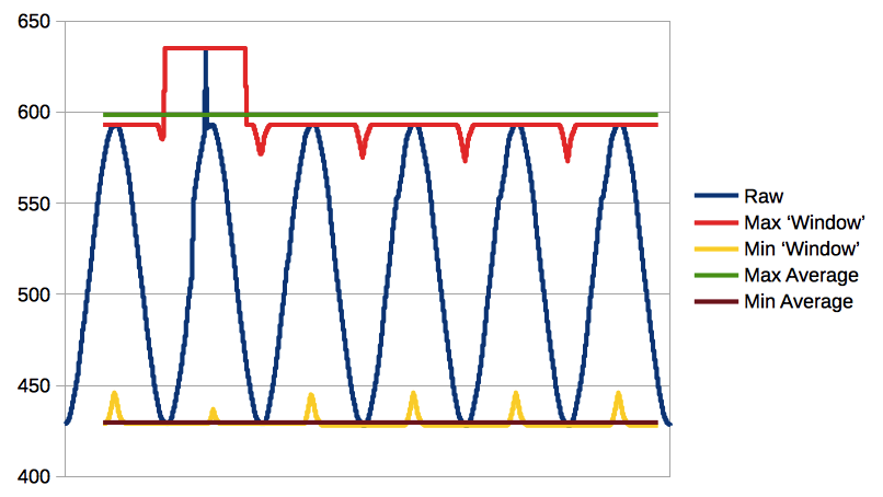
To make a shorter list of numbers, we can take out unnecessary information from our sine wave. The ‘unnecessary’ information is basically ‘anything that isn’t a peak or a trough’ since those are the only points we care about to calculate amplitude.
We could just take the highest and lowest points of the entire 7500 item list and call it a day, but this might be a problem when there are outliers or measurement errors that are sudden spikes in the data. So we want to amplify the effect of peaks and troughs, but smooth out the effect of any one outlier peak or trough.
Make a sliding ‘window’ and every 100 measurements, find the max and min value of the 50 preceding and 50 next measurements.
Taking the average of these ‘windowed’ amplitudes means that any one accidental spike will only count toward the average of its own peak or trough, and the rest of the wave cycles will push the average closer to its true value.
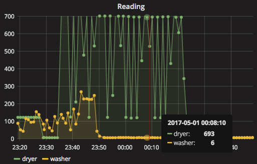
Notice how, in this image, a single spike makes the global maximum around 625 while the true maximum, seen over several cycles, is closer to 595. Using the ‘window’ approach pulls the average maximum closer to its true value.
To get from an average peak / trough to an average amplitude is as easy as subracting the trough from the peak.
Finally, we come to our measurement algorithm: a function that starts off by measuring each channel 7500 times at 50 kHz and spits out a single number - an adjusted-average amplitude.
defmeasure(number):ch0list=[]ch0avg=[]for_inrange(1,number):#Measure n times
ch0list.append(read_mcp3002(0))forstepinrange(50,(number-50),100):# Make peak/trough windows
ch0max=max(ch0list[step-50:step+50])ch0min=min(ch0list[step-50:step+50])ch0avg.append((ch0max-ch0min))ch0=reduce(lambdax,y:x+y,ch0avg)/len(ch0avg)#Calculate the average amplitude
returnch0printmeasure(7500)
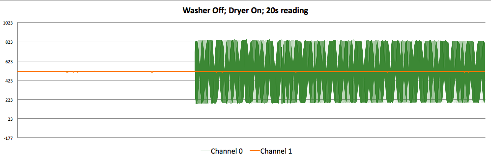
Let’s have a look at some real-life amplitude measurements during a washer and dryer cycle:
At rest, each appliance usually has an average-adjusted amplitude of 6.
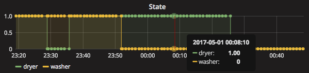
From Amplitude to State, and Keeping Track of State
So then, to get from amplitude to appliance state is not a taxing calculation: Any amplitude greater than 12 is ‘on’, anything 12 or less is ‘off’
We set up our measurement script to run once every minute and find the current state of the appliance. But the script only knows what the appliance is doing this very minute. How can we find out what it did in the previous minute?
For that, we’ll need a database. InfluxDB is a great choice for this application, as it’s designed for measuring things over time.
So to add to our script that runs each minute, we’ll write the measurement and state to the database:
#!/usr/bin/python
frominfluxdbimportInfluxDBClientUSER='root'PASSWORD='root'DBNAME='db'HOST='hostname'PORT=8086client=InfluxDBClient(HOST,PORT,USER,PASSWORD,DBNAME)client.create_database(DBNAME)client.switch_database(DBNAME)mm=measure(7500)# As defined above
statemin=12state=1if(mm>statemin)else0newpoint=[{"measurement":"voltage","fields":{"washer":mm}},{"measurement":"state","fields":{"washer":state}}]client.write_points(newpoint)
We can now keep track directly of when an appliance is on or off:
Comparing States and Taking Actions
Now we can compare the current state to the previous state.
Most of the time, we’ll find that the state is unchanged. An appliance in motion tends to remain in motion, and an appliance at rest tends to remain at rest. But occasionally, we’ll find that the state is different - the appliance started up or the appliance powered down.
So we have to get the last known state:
#!/usr/bin/python
query="SELECT * from state GROUP BY * ORDER BY DESC LIMIT 1"result=client.query(query)resultlist=list(result.get_points())lastknownstate=resultlist[0]['washer']
Now we compare the last known state to the current state:
There are two possible state transitions: ‘on’ to ‘off’ and ‘off’ to ‘on’. We’ve called these ‘powering up’ or ‘shutting down’. I only want to get text messages when an appliance shuts down - after all, when it turns on someone is standing there pushing the ‘on’ button.
To get text messages from our Python script we’ll use the awesome Twilio Python REST API.
#!/usr/bin/python
importdatetimefromtwilio.restimportTwilioRestClientimportpytzfromdatetimeimportdatetimeaccount_sid="xxxxxxxxxxxxxxxxxxxxxxxxxxxxxxxx"# Your Account SID from www.twilio.com/console
auth_token="xxxxxxxxxxxxxxxxxxxxxxxxxxxxxxxx"# Your Auth Token from www.twilio.com/console
twilioclient=TwilioRestClient(account_sid,auth_token)numbers=["+15555555555","+15555554444"]# Your intended SMS recipients
currenttime=datetime.now(pytz.timezone('US/Central')).strftime('%-I:%m %p')# The time like '6:10 PM'
if(currentstate!=lastknownstate)andcurrentstate==0:#Only do this when the appliance turns off
forninnumbers:twilioclient.messages.create(body=("💧 Washer is done! "+currenttime),to=n,from_="+15555553333")# Replace with your Twilio number
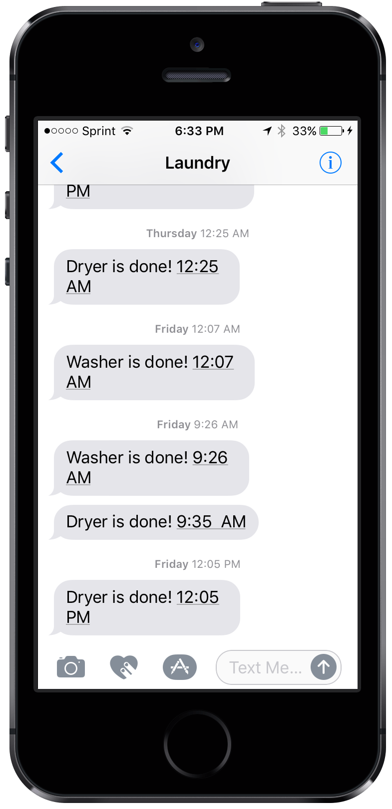
Now I’m happily enjoying my laziness and a prompt turnaround on laundry:
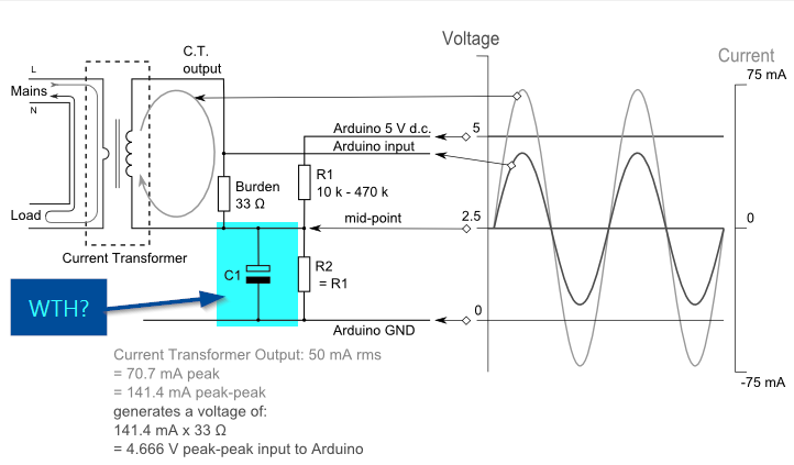
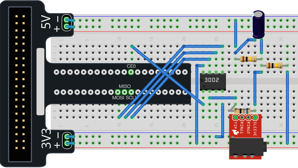
When I was following the OpenEnergyMon guide I noticed they were including a capacitor in their circuit:
What’s that there for? It’s to provide an alternative path for some of the current to flow to the ground. Capacitors take some time to charge up and then discharge all at once, in a way that is dependent on the frequency of the current flowing through them. An arrangement like this with a resistor and a capacitor together is called a low-pass filter, meaning that only signals with a low frequency will be able to pass. It will filter out excess noise.
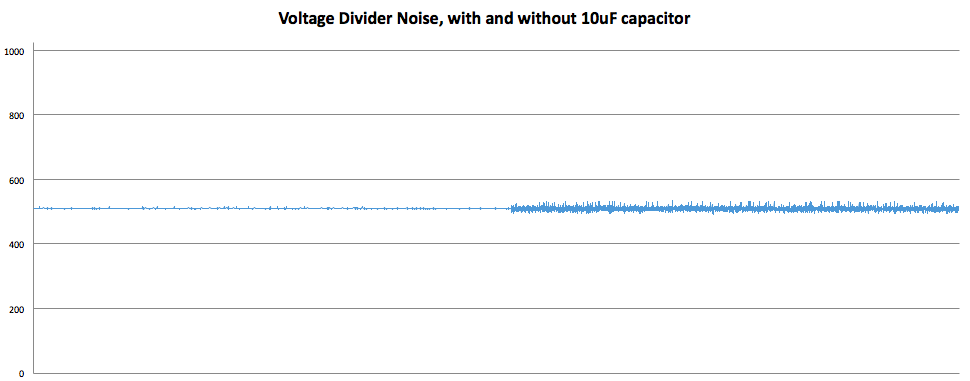
I did some experimenting by measuring the voltage signal with and without the low-pass filter.
Across the entire range of the ADC:
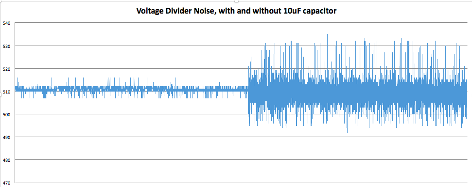
and zoomed in:
As you can see, it’s not trivial. A perfectly clean signal would measure 511 every time, but there’s some jitter. With the low-pass filter, the difference between the maximum value and the minimum is around 15. Without the filter, it’s much as 50. To a crude approximation, the filter adds around 10% accuracy to our measurement.
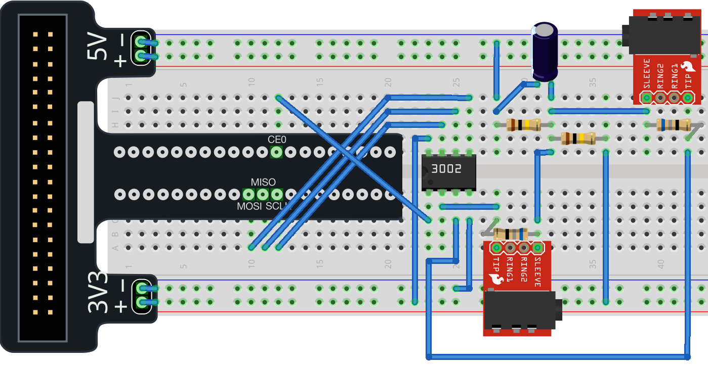
Two Jacks and Two Channels
Up to this point, we’ve only been measuring one input at a time. With 2 channels, the MCP3002 can read 2 voltages. And with 2 laundry appliances, that’s what I need to do.
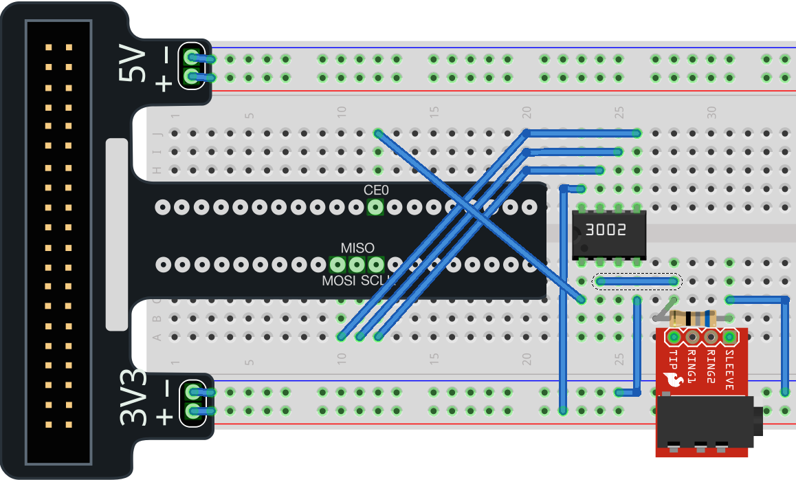
We’ll add a second jack to the circuit:
We can share the same voltage divider, and direct our output to channel 1.
Measuring the Real Appliances
Now, in order to translate voltage readings into the state of the appliance, I need to actually measure the appliances. I turned the breaker off to the dryer, unplugged it, and took off the back cover to fit the current sensor around 1 of the wires. A 220V dryer in the US has 4 wires coming into it. The green ground, 2 phases of power (red and black) and a white neutral. After some trial and error, I found that my dryer had the heating element powered by the left phase and the motor powered by the right phase.
For the washer, I turned off the breaker to the outlet it was plugged into and put the current sensor around the power line inside the outlet.
I cued up the measurement script and took some readings of the dryer:
It was basically perfect. I was excited here - the washer reading stays almost exactly at baseline and the dryer reading starts out there. When the dryer turns on, it is instantaneously recognizable in the graph.
In Part 5, I’ll show you my algorithm for turning thousands of measurements into a single meaningful data point.
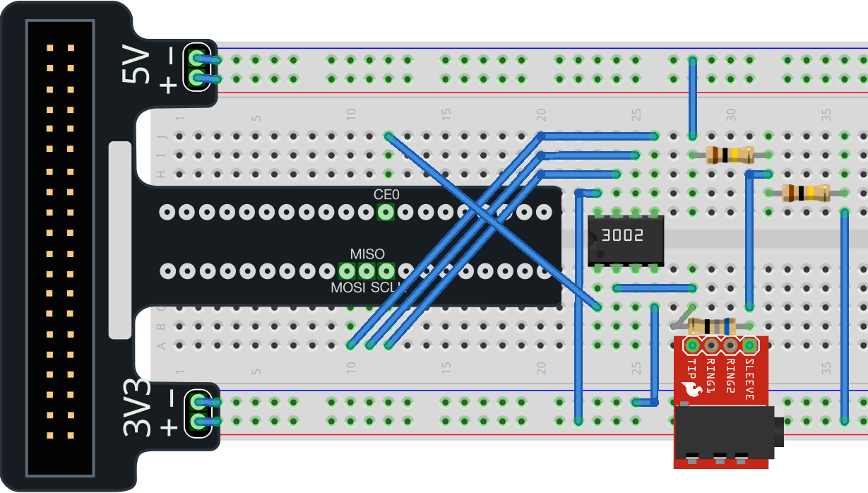
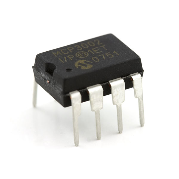
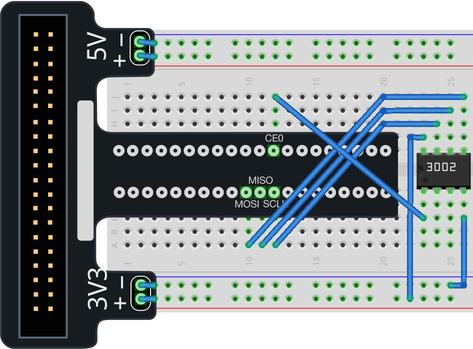
We’re using the SPI interface, so we want to hook up the Pi to the MCP3002 like so (note the little divot on the left side of the MCP3002 for alignment):
MCP3002
RPi
Reason
VDD
3V3 +
Operating voltage; max voltage
CLK
SCLK
Clock sync
DOUT
MISO
Data out of the MCP3002 and into the Pi (Master In; Slave Out)
DIN
MOSI
Data into the MCP3002 and out of the Pi (Master Out;Slave In)
CS
CE0
Chip Select - there are 2 data channels on the Pi and we’ll use the first one, 0
VSS
GND (3V3 - )
Ground (On the CanaKit breakout, it’s also called “3V3 -“
This leaves 2 pins unconnected on the MCP3002 - CH0 and CH1 - the 2 channels of data we can measure. Let’s leave them empty for now.
Programming the Pi
Now we can finally measure using the Pi. Boot into your Pi and get it into SPI mode:
#!/usr/bin/python
#-------------------------------------------------------------------------------
# Name: MCP3002 Measure 3V3
# Purpose: Measure the 3V3 Supply of the Raspberry Pi
#-------------------------------------------------------------------------------
importspidev# import the SPI driver
fromtimeimportsleepDEBUG=Falsevref=3.3*1000# V-Ref in mV (Vref = VDD for the MCP3002)
resolution=2**10# for 10 bits of resolution
calibration=0# 38 # in mV, to make up for the precision of the components
# MCP3002 Control bits
#
# 7 6 5 4 3 2 1 0
# X 1 S O M X X X
#
# bit 6 = Start Bit
# S = SGL or \DIFF SGL = 1 = Single Channel, 0 = \DIFF is pseudo differential
# O = ODD or \SIGN
# in Single Ended Mode (SGL = 1)
# ODD 0 = CH0 = + GND = - (read CH0)
# 1 = CH1 = + GND = - (read CH1)
# in Pseudo Diff Mode (SGL = 0)
# ODD 0 = CH0 = IN+, CH1 = IN-
# 1 = CH0 = IN-, CH1 = IN+
#
# M = MSBF
# MSBF = 1 = LSB first format
# 0 = MSB first format
# ------------------------------------------------------------------------------
# SPI setup
spi_max_speed=1000000# 1 MHz (1.2MHz = max for 2V7 ref/supply)
# reason is that the ADC input cap needs time to get charged to the input level.
CE=0# CE0 | CE1, selection of the SPI device
spi=spidev.SpiDev()spi.open(0,CE)# Open up the communication to the device
spi.max_speed_hz=spi_max_speed#
# create a function that sets the configuration parameters and gets the results
# from the MCP3002
#
defread_mcp3002(channel):# see datasheet for more information
# 8 bit control :
# X, Strt, SGL|!DIFF, ODD|!SIGN, MSBF, X, X, X
# 0, 1, 1=SGL, 0 = CH0 , 0 , 0, 0, 0 = 96d
# 0, 1, 1=SGL, 1 = CH1 , 0 , 0, 0, 0 = 112d
ifchannel==0:cmd=0b01100000else:cmd=0b01110000spi_data=spi.xfer2([cmd,0])# send hi_byte, low_byte; receive hi_byte, low_byte
# receive data range: 000..3FF (10 bits)
# MSB first: (set control bit in cmd for LSB first)
# spidata[0] = X, X, X, X, X, 0, B9, B8
# spidata[1] = B7, B6, B5, B4, B3, B2, B1, B0
# LSB: mask all but B9 & B8, shift to left and add to the MSB
adc_data=((spi_data[0]&3)<<8)+spi_data[1]returnadc_datatry:print("MCP3002 Single Ended CH0,CH1 Read of the 3V3V Pi Supply")print("SPI max sampling speed = {}".format(spi_max_speed))print("V-Ref = {0}, Resolution = {1}".format(vref,resolution))print("SPI device = {0}".format(CE))print("-----------------------------\n")whileTrue:print(read_mcp3002(0),read_mcp3002(1))exceptKeyboardInterrupt:# Ctrl-C
spi.close()defmain():passif__name__=='__main__':main()
run it, and you should see output like this:
MCP3002 Single Ended CH0 Read of the 3V3 Pi Supply
SPI max sampling speed = 1000000
V-Ref = 3300.0, Resolution = 1024
SPI device = 0
-----------------------------(0,0)(0,0)(0,0)(1,0)(0,0)(0,2)(0,0)(0,0)
Since no current is flowing through the CH0 and CH1 pins, they are essentially at zero volts. There can be some error in the measurement, but it’s close enough.
Measuring Some Voltage
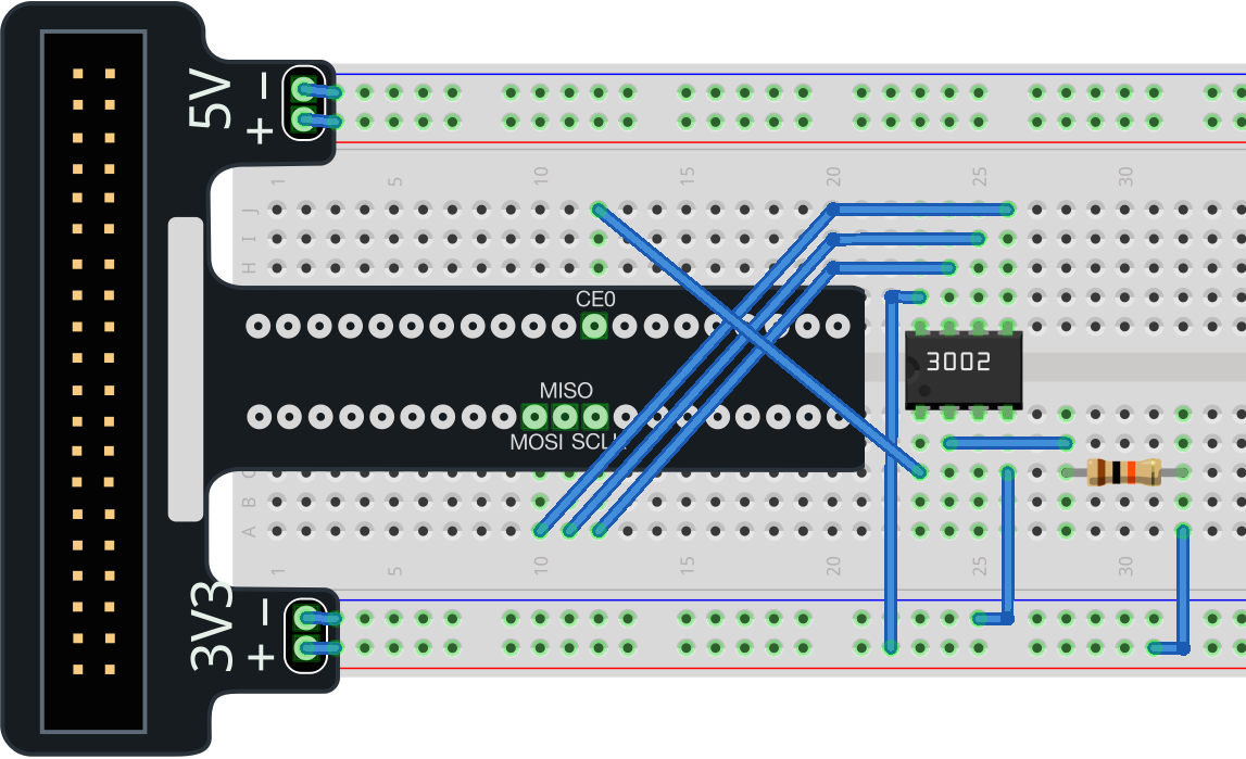
Cool, now let’s see the high end of the scale. We can measure up to 3.3V. Let’s hook up CH0 to the 3V3 rail with a 10kOhm resistor to prevent damaging the Pi:
Measure again:
MCP3002 Single Ended CH0 Read of the 3V3 Pi Supply
SPI max sampling speed = 1000000
V-Ref = 3300.0, Resolution = 1024
SPI device = 0
-----------------------------(1023,0)(1023,0)(1023,0)(1023,0)(1023,0)(1023,0)(1023,0)
Cool, we’ve measured the top of the range and the bottom of the range!
Let’s measure some real voltage from the CT sensor:
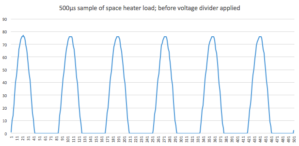
Now, the CT sensor is connected to GND across a 68 Ohm resistor. When no current flows through the CT sensor, we will read 0V. We put the CT sensor around a 12A space heater and echo the output of the measure program to text:
python measure.py >> heater.txt
I took that and plotted it in Excel:
One thing to notice is that we’re only getting half of the information about the AC wave. This is because when the wave is at its peak, we’re pushing voltage toward the GND pin. When the wave is in a trough, it’s trying to push voltage back toward the 3V3 pin to no avail and the MCP3002 still reads it as 0V.
We need to get the steady-state voltage up to a higher amount so that we can still read a positive voltage with the MCP3002. How about halfway?
Voltage Divider
Resistors create something called a “voltage drop” which is some EE wizardry that I don’t understand. Take it for granted that when you have a resistor, the voltage on one terminal is measurably and proportionally different to the voltage on the other terminal. We can exploit this principle to put our circuit at that “steady state” I mentioned before.
By connecting two resistors in series and then measuring the voltage in between them, we can obtain a desired voltage that is a specific fraction of the input voltage. This arrangement is called a voltage divider.
From the equations there, we postulate that if we have 2 resistors of equal resistance connected in series, then the voltage between them will be exactly half the input voltage.
R1 = R2 = 100kOhm
I’ll use 100kOhm resistors to lessen the amount of current this circuit will drain from the Pi in case I use a battery pack.
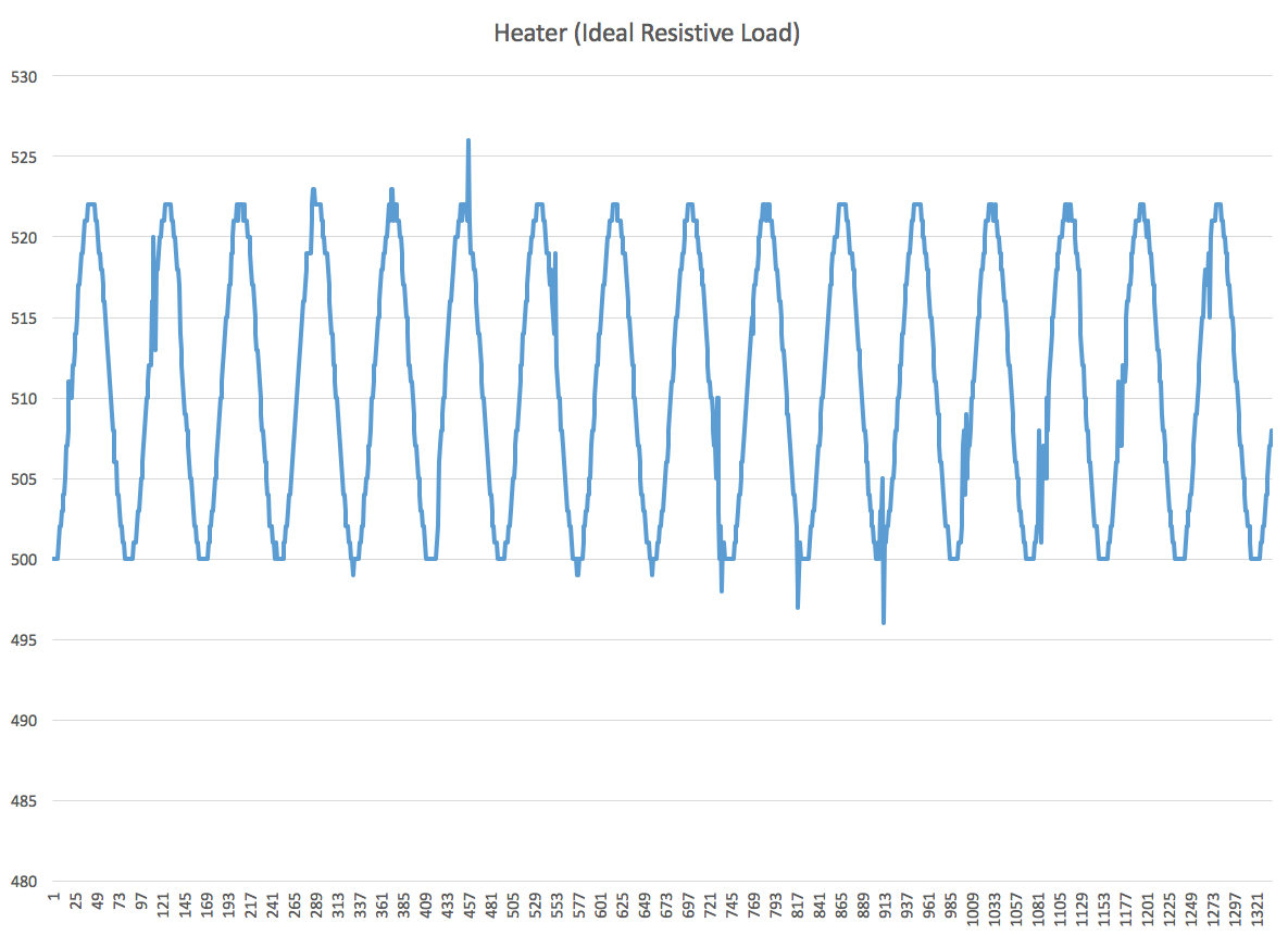
Let’s measure the heater again:
Cool. We can now see the full AC sine wave of this space heater - which is an ideal resistive load, always using a consistent amount of power. You’ll noticed it’s centered around 1/2 of our 10-bit scale: 511.5.
You’ll notice that these come with 3.5mm TRS plugs on the end. This will make them easy to plug in and remove, but now I need a jack to receive them.
SparkFun TRRS 3.5mm Jack Breakout
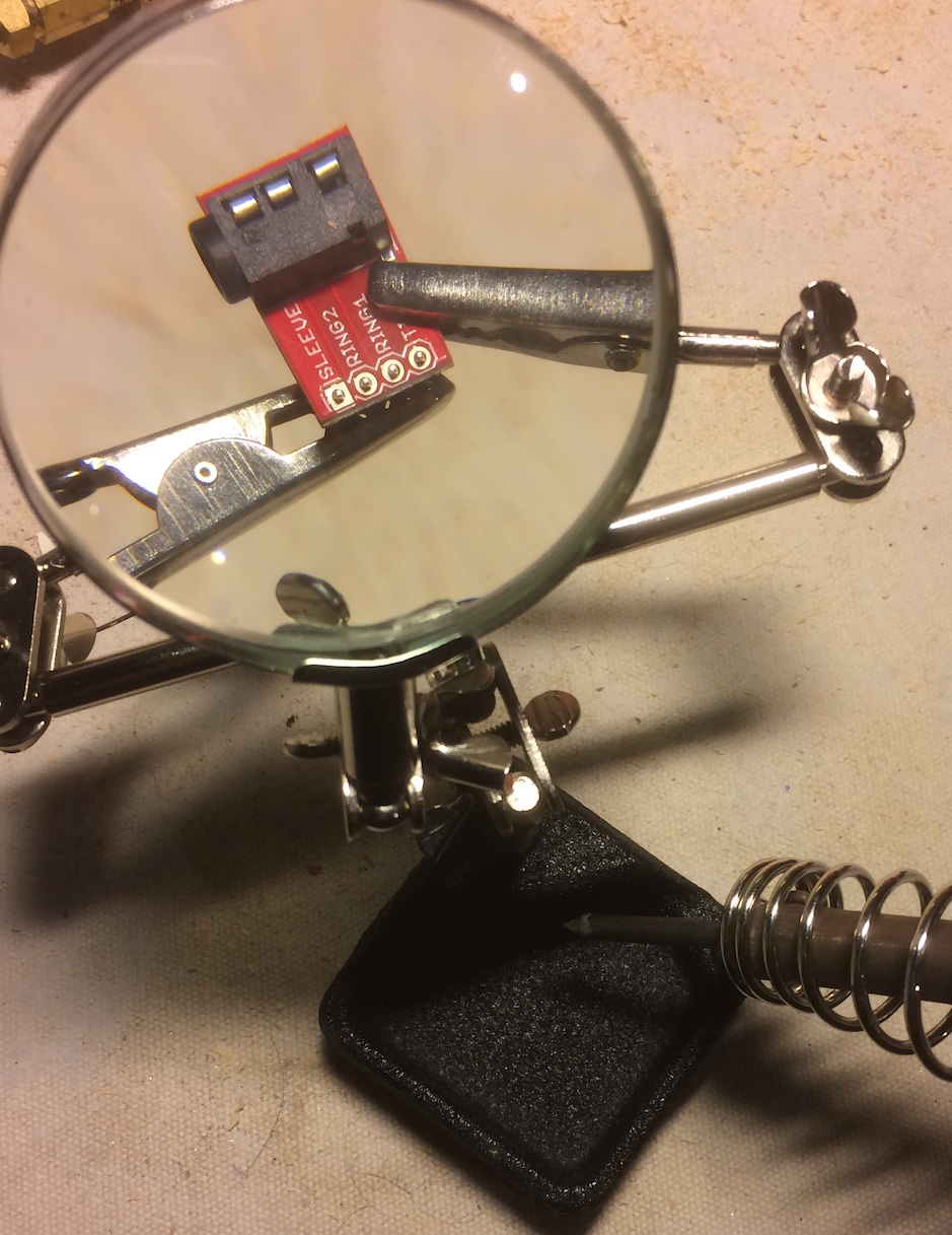
These jacks come already assigned to a breakout board, which will make it convenient to use them with a breadboard - once some headers are soldered on:
Break Away Headers - Straight
Once the parts arrived, I needed to solder the header pins onto the jack breakout for attaching to the breadboard. I’d never soldered delicate electronics, only larger wires so I picked up some 0.32 solder and watched some tutorials.
With the parts soldered and prepared, it’s time to start measuring.
Measuring Current
So a little math here. According to the datasheet, our current sensor has a 2000-turn ratio. This means a current of 30 Amps, divided by 2000 turns, will yield a resultant current of 15mA. What voltage will that current be at? Well, theoretically, an infinite voltage (I don’t quite understand why this is, but I trust the opinion of people smarter than me). If you just hook the CT up to a multimeter, that meter will have resistance in the circuit and so you’ll get a “voltage drop” across the two leads of the multimeter.
And so we get to measuring a 100-Watt lightbulb with just the multimeter hooked to it for a test. Turns out, with a measly 0.8 A of current, we’re already up to 2V. This won’t do. I need a way to get the voltage down further.
The key bit is that our maximum measurable voltage is 3.3V - that’s the potential we’re feeding into the MCP3002. Since we’re measuring AC current, it means that 3.3V is the peak-to peak meaning that we actually want to measure a max of 1.65V as our zero-point or reference point. At the maximum peak of the AC wave, we’ll have 1.65V reference + 1.65V from the sensor = 3.3V. At the minimum trough of the AC wave, we’ll have 1.65V - 1.65V = 0V.
The equation for burden resistor calculation is:
With a 30A current, we’d have a burden resistor value of 38.8 Ohms.
Since RadioShack had 68 Ohms as the closest resistor value (heh), I can actually measure up to 17A safely:
So we have a circuit that won’t overvolt the Pi! In part 3, we’ll hook the sensor up to the Pi and start measuring it.


 R1 = R2 = 100kOhm